Coarsening and Extrusion
After segmenting the images and identifying the electromagnetic materials, a voxel model can be obtained by extruding each pixel in the +z and –z directions. This results in a very large dataset that can be used only by a few electromagnetic simulators at this time. To enable quicker (but less accurate) analysis, this data set was ‘coarsened’ and smaller models were developed. Various different approaches can be used for obtaining coarser models; as detailed below, two different methods were used for the AustinMan models: A 2-D coarsening method was used for the AustinMan v1.0 model and a 3-D one was used for the AustinMan v1.1, AustinMan v2.0, and following models. The 2-D coarsening method discards some of the slices and does not rely on/take advantage of the information in those slices, whereas the 3-D coarsening method uses information from all the slices. The 2-D coarsening method can be used to create models even when not all the slices are segmented whereas the 3-D results in more accurate models.
2-D Coarsening: AustinMan v1.0
In the 2-D coarsening method, first the z-direction is coarsened by discarding image slices, e.g., to create the 4×4×4 mm3 AustinMan v1.0 model, slices 1002, 1006, 1010, etc. were kept and slices 1003-1005, 1007-1009, etc. were discarded. Then, the pixels in each of the remaining slices are coarsened independently by combining multiple pixels to create larger pixels (starting the combination from the (x,y) = (1,1)pixel [top left corner of the cropped image] of each slice and shifting): Each new pixel is assigned a material by finding the mode of the materials (the most frequent material) in an area of pixels. For example, for the 4 × 4 × 4 mm3 resolution model, all pixels in an image slice are grouped into 12 × 12 sets of (1/3 × 1/3 mm2 ) pixels and each 12 × 12 set of pixels is replaced with a single 4 × 4 mm2 pixel. If the 12 ×12 set of pixels consisted of 35 pixels of Vacuum, 42 pixels of SkinDry, 56 pixels of Fat, and 11 pixels of Muscle, then the new pixel would be considered Fat. In the rare instances where two or more materials had the same number of pixels in an area, the material with the lowest material id number in the electromagnetic materials table was chosen (essentially a random choice among the materials). Once the larger pixels are created they are extruded Δz/2 in the +z and –z directions to create cubic voxels. Note that, to keep the top and bottom of the different resolution models at the same location, the first and last slices (slices 1002 and 1354) were extruded Δz/2 only in the –z and +z directions, respectively. As a result, the voxels at the top and bottom of the model are half as high as the remaining voxels (Fig. 1).
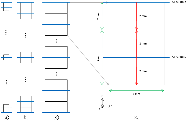
Figure 1: 2-D coarsening. The (a) 1 × 1 × 1 mm3, (b) 2 × 2 × 2 mm3, and
(c) 4 × 4 × 4 mm3 voxel resolutions in the AustinMan v1.0 model.
The blue lines represent the image slices while the black lines
represent the boundaries of the voxels. (d) A zoomed-in version of
the top of the 4 × 4 × 4 mm3 resolution model that shows how the
top slice is only extruded downward 2 mm (Δz/2). The red arrows
indicate the direction and distance that each slice was extruded
and the green arrows indicate voxel dimensions.
3-D Coarsening: AustinMan v1.1 and Later
In the 3-D coarsening method, first pixels are extruded in the z-direction to create 1/3 × 1/3 × 1 mm3 voxels. Then, the voxels are coarsened by combining multiple voxels (starting from the top left corner of the top slice, i.e. (x,y,z) = (1,1,1) voxel of the model): Each new voxel is assigned a material by finding the mode of the materials (the most frequent material) in a volume of voxels. For example, for the 4 × 4 × 4 mm3 resolution model, the voxels are grouped into 12 × 12 × 4 sets of (1/3 × 1/3 × 1 mm3) voxels and each 12 × 12 × 4 set of voxels is replaced with a single 4 × 4 × 4 mm3 voxel (Fig. 2). Note that unlike the 2-D coarsening the pixels in the first and last image slices are extruded both up and down 0.5 mm for the initial (finest resolution) model. This method ensures that each of the initial voxels is given equal weight during coarsening and that the top and bottom of the model has the same locations regardless of the resolution. Note that when the number of image slices is not a multiple of the coarsening factor, the height of the voxels at the bottom are set to the height of the remaining slices and the voxels at the bottom of the coarsened model have a different height than the rest. For example, if there are 353 image slices in the finest-resolution model, then the voxels at the bottom of the 1 × 1 × 1 mm3 , 2 × 2 × 2 mm3 , and 4 × 4 × 4 mm3 resolution models would have sizes of 1 × 1 × 1 mm3, 2 × 2 × 1 mm3, and 4 × 4 × 1 mm3, respectively.
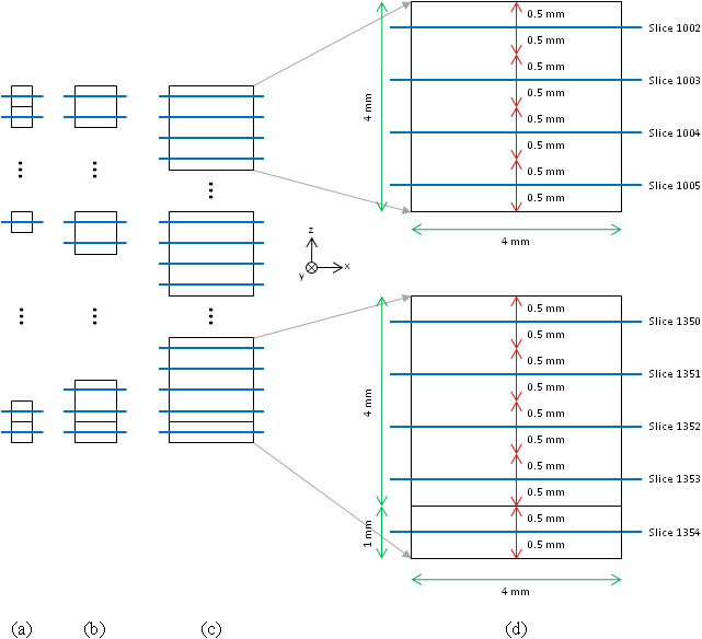
Figure 2: 3-D coarsening. The (a) 1 × 1 × 1 mm3,
(b) 2 × 2 × 2 mm3, and (c) 4 × 4 × 4 mm3 voxel resolutions in the
AustinMan v1.1 model. The blue lines represent the image slices
while the black lines represent the boundaries of the voxels. (d) A
zoomed-in version of the top and bottom of the 4 × 4 × 4 mm3 voxel
resolution model. Notice that the voxels at the bottom can have a
different height than others. The red arrows indicate the direction
and distance that each slice was extruded and the green arrows indicate
voxel dimensions.
| Previous: Segmentation and Material Identification | Up: Methodology |
